Necessary Conditions for Robust Fundamental Parameter
Analysis in EDXRF
John Maxwell
&
Tibor Papp
Cambridge Scientific, Guelph, ON, Canada
 |
EDXRF – Energy Dispersive X-Ray Fluorescence
FP – Fundamental Parameter – so called because it uses a physics database of the fundamental physical parameters such as ionization cross-section, mass attenuation coefficients, line energies and relative line intensities etc. to calculate theoretical yields in order to first fit elemental peak areas and then convert fitted peak areas to elemental concentrations
- we will start with a quick review of the general requirements to perform pure or standardless FP calculations
- from there we will proceed to a description of what we will term Hybrid FP or FP done with standards that are used to characterize the system and how these standards loosen the stringent “know everything” requirements of pure FP
Block Diagram of EDXRF Setup
X: x-ray
source
P:
Pre-filter (if any) 1: where source x-rays strike sample 2:
where sample x-rays leave surface A: x-ray absorbers (if
any)
D:
detector PA:
pre-amplifier
SP:
signal processor C: computer for displaying & analyzing spectrum
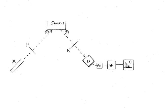
(1) Spectrum of x-rays striking the sample
(2) Spectrum of x-rays leaving the sample in the direction of the detector
We must examine the basic assumptions and what happens at each point in the apparatus to determine what is important to obtain a robust (repeatable and accurate) measurement and spectrum analysis.
Determining Elemental Concentrations Via FP Analysis
In its simplest form we have the equation
C(Z) = A(Z,True) / Y(Z,M,d,N(E),G) (1)
where
A(Z,True): actual or “true” number of x-rays/second of the principal line of element Z (line type K, L, M) leaving the sample surface in the direction of the detector [ point 2 in the block diagram].
Y(Z,M,d,N(E),G): theoretical calculation of the number of x-rays.second of the principal line of element Z (K, L or M) leaving the sample surface in the direction of the detector
This is a very simple equation with a great deal hidden in the details.
Determining A(Z,True)
This is the sample spectrum at point 2 in the block diagram (the spectrum of x-rays leaving the sample in the direction of the detector) and determining this spectrum from the recorded spectrum is not as easy as one might assume:
- what the analyst sees and has to work with is the x-ray energy spectrum recorded and displayed in the computer
- the x-ray energy spectrum at point 2 is modified by all x-ray attenuators located between the sample and the detector with the attenuation being x-ray energy dependent – call this term Abs(Z)
- the spectrum entering the detector is further modified by detector windows and electrodes before entering the detector crystal
- within the detector crystal many things occur to modify the energy signal but in simple terms each x-ray that interacts within the crystal volume, and not all do as some may traverse the entire crystal without interaction, will produce a signal proportional to the energy deposited in the crystal. The end result is that each x-ray results in the production of electron-hole (e-h) pairs with the number of such pairs proportional to the energy deposited. However, there are mechanisms for loss due to energetic electron escape, the escape of detector element x-rays, charge trapping etc. that result in a smearing out of the line shape.
- Electrical noise and the statistical nature of the e-h production process results in a broadening of the main peak, which is usually assumed to be Gaussian but is better represented by a Voigtian profile to account for the natural line width of the characteristic x-rays.
- As a result of the losses and broadening a narrow x-ray line results in an observed signal showing a broadened main peak with low energy structure that can include short and long range tailing features and escape peaks characteristic of the detector material.
This is represented pictorially below
Monoenergetic Cu Ka1
x-rays produce Þ
|
Monoenergetic Cu Ka1 x-rays produce Þ |
 |
Observed Signal
This represents a very simplified view of what occurs in the detector and the details would have to be the subject of a different discussion.
All of these detector factors combined
- attenuation in the windows & electrode material
- fraction lost because they traverse the crystal without depositing energy
- the fraction lost to lower energy that show up as tailing and escape peaks
will combine together into a term we will call the intrinsic detector efficiency, Dint(Z) , which represents that fraction of events that produce a full energy signal in the pre-amp trace.
The preamplifier signal now enters the processing electronics, whether analog, digital or some combination of the two, where it undergoes further modification.
The Processor:
The main job of the processor is to recognize the signature of an event in the pre-amp trace and determine its amplitude (which will be proportional to the energy of the originating event) in order to place it into the observed spectrum.
The main effects that the processor has on the signal include:
- at low energies it can be difficult to distinguish true events from the noise (signal recognition efficiency)
- the finite time required to process an event can result in partial or full signal pile up resulting in sum peaks as well as partial energy structures between the main parent event peaks and the sum peak
- component dead time (whether preamp, processor, ADC etc) results in the loss of events
- if discriminators are used to improve the spectral quality by eliminating noisy or poor quality events then there may be an energy or spectral dependence to the rejected events
We combine all of these factors together into a term we will call the electronic detection efficiency, Delec(Z).
This value will be rate, spectral, noise and possibly energy dependent.
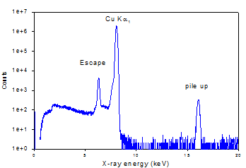
Cu Ka1 line from an x-ray monochromator Upper panel. The total spectrum, with
no discrimination
Middle panel: the “desirable” or
accepted spectrum passing through some
selection criteria
Lower panel: that part of the total spectrum
rejected by some criteria Observe the sum peak in the accepted spectrum as well as both pile-up peaks and continuum in the total and
rejected spectra. Also observe the rejected
low energy noise peak.
Many
of the electronic effects are shown in spectra collected with a CSX processor
 |
Putting this all together we can obtain the adjusted peak area leaving the sample (point 2 in the block diagram] to be
A(Z,True) = (Fitted spectrum peak area) / [ Abs(Z) * Dint(Z) * Delec(Z) * t ]
Where t is the measurement time in seconds,
Abs(Z) is the fraction transmitted through the x-ray attenuators
Dint(Z) is the fraction of events striking the detector that show up with full energy signatures in the pre-amp signal
Delec(Z) is the fraction or full energy preamp events that show up in the observed spectrum in the main peak, not as a degraded or pile up event.
FP is also useful in determining the “Fitted Spectrum Peak Area”
Fitted Spectrum Peak Area
In simple spectra, with well-separated peaks and no background, peak intensities can be estimated accurately by summing over regions of interest (ROI) for each peak.
Adding background complicates the procedure as the background under the peak needs to be estimated and subtracted from the peak intensity. In its simplest form, this is often accomplished by estimating the background to the left and right of the peak and making the appropriate subtraction in the peak region.
As spectra become more complex and one peak structure begins to overlap another peak structure these simple procedures are no longer adequate.
This is where FP can be useful. An FP database can be used to obtain the relative line intensities for each series of x-rays for each element (K, L or M). These line intensities are modified relative to one another for thick target, absorber and detection efficiency effects via FP calculations.
A model spectrum can be built and fitted to the observed spectrum with the fitted intensities providing the necessary estimates of the principal line peak area. Overlaps from lines of one element with another can often be adequately handled in this manner. Each element has more than one line with their relative intensities known, which provides a basis for separating the intensities of the overlapping peaks.
This takes care of the 1st term in Eq (1) - so now we have to deal with the 2nd term, the calculated theoretical yield term Y.
Theoretical Yield
Y(Z,M,d,N(E),G) – is the calculated x-rays per second leaving the sample surface in the direction of the detector crystal
M: represents the sample matrix effect on the yield calculation,
d: represents the sample thickness either in length or areal density units
N(E): is the number of source x-rays striking the sample/second as a function of energy E at point (1) in the block diagram. Often the energy spectrum is given in binned form allowing sum calculations as opposed to integral calculations.
G: the geometry of the measurement that includes the angle the source beam makes with respect to the sample surface, the angle the sample x-rays make with respect to the detector crystal and the solid angle the detector crystal makes with respect to the sample.
Geometry Diagram of Source-Sample-Detector Geometry
X: x-ray
source
d:sample thickness (areal
density)
D: detector C: detector crystal a: angle between
source x-ray beam and sample normal q: angle between
sample normal and detector normal
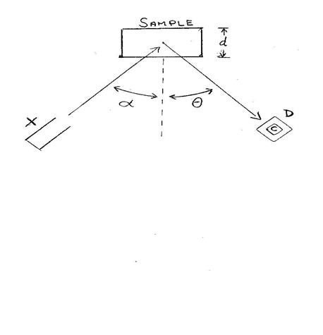
- The angles a, q define the path that the source and sample x-rays take within the sample. In thick targets both of these angles are important, as errors in these angles will result in incorrect path lengths and calculated yields.
- In thin targets, where there is no thick target correction, only a is important as the path experienced by the source x-rays is not d but is instead d/cosa.
- The solid angle in steradians the detector crystal (C) makes with respect to the sample is essentially the detector crystal (collimated) area divided by the square of the distance from the sample surface to the crystal surface.
- Whether a thin or thick target, the solid angle is important as it determines the fraction of events that could be detected. This value is often ignored but shows up in either the instrument calibration factor or the overall source beam intensity. However, it is better to include it explicitly as it can point to issues with the measurement.
- In some cases the solid angle can be complicated to calculate when the detector is placed close to the sample and the sample is light enough and thick enough to have a significant depth profile to its yield as the x-rays originating from a greater depth will have a smaller solid angle of detection.
- The sample thickness d is one of the variables that must be known, measured or calculated in x-ray fluorescence analysis. Sample thickness is defined here as areal density (g/cm2). It is not sufficient to know or measure the thickness in cm (mm or mm) it is necessary to also know the sample material density as it is the areal density that is used to calculate the attenuation of x-rays, both source and sample, in the sample material.
- For very thin samples the yield is essentially linearly proportional to the areal density, however as the sample thickens the incremental yield decreases exponentially until you reach the “thick” target status and there is no increment in characteristic x-ray yield with further thickening of the sample.
- If the sample is sufficiently thick such that the source x-rays are totally attenuated by the sample or at least the sample x-rays of interest cannot penetrate the entire thickness then knowing the actual areal density or thickness is usually not necessary. The exception to this rule is in light element matrices where 10 keV x-rays may penetrate several mm and 25 keV x-rays may penetrate several cm resulting in a changing solid angle of detection in typical set-up geometries.
- This table shows estimates of depths by which 50% or 90% of the total yield will have occurred for x-rays of various energies in a gold, iron or polyethylene samples.
keV Iron Gold Polyethylene (C2H4 0.92g/cm3 )
50% 90% 50% 90% 50% 90%
mm mm mm
5 6.3 21 0.5 1.8 0.5 1.5
10 5.2 17 3.0 10 3.6 12
15 15 51 2.2 7.3 10 33
20 34 110 4.6 15 17 58
25 64 210 8.1 27 23 78
30 110 360 13 43 28 93
- for medium to high Z samples the analysis depth is measured in mm. This means that samples of the order of one mm thick would be considered thick targets in most of these cases and the actual analysis depth often does not exceed more than a few mm .
- the table indicates that in low Z element samples the targets are often not “thick” unless they exceed many cm’s which is rarely the case. Also the densities of many plastics depend on the manufacturing process so that it is the responsibility of the analyst to know the basic structure of the material they are analyzing including its density and thickness or simply areal density.
The Sample Matrix Effect (M)
The sample matrix, or bulk non trace composition, is important as it is the matrix that determines
- The path length of interaction of both the source and sample x-rays via the energy dependent mass attenuation coefficients.
- Whether secondary x-ray production processes, especially secondary fluorescence, is important for each element Z
- Trace constituents, below about 1 part per thousand, have little effect on either of these factors
Other sample considerations include
- rough or curved surface effects
- sample preparation as necessary to ensure a homogeneous matrix
The Source X-Ray Spectrum
Source x-rays are usually produced in one of four ways
- radioactive isotope source whose line energies and relative line intensities are generally well known
- synchrotron radiation with the x-ray spectrum depending upon the tuning
- fluoresced x-rays from a secondary target
- x-ray tube radiation with characteristic lines from the anode material, (and a possible pre-sample filter material), as well as a continuum bremsstrahlung spectrum as a result of the electron braking in the tube anode
In most analytical instruments, x-ray tubes, with or without pre-filters or secondary targets provides the primary source of x-rays.
With x-ray tubes defining the “EXACT” spectral shape and intensity striking the sample is problematical.
Why is this important?
FP calculations rely on calculated x-ray production yields with one of the factors being the energy dependent ionization cross-sections.
These cross-sections essentially decrease rapidly above the shell binding energy except in the energy region just above the edge (dashed line circled region) where oscillatory fine structure effects can occur (XAFS or XANES & EXAFS) – but this is beyond the scope of this discussion.
Figure of ionization cross-section (ICS) vs
Energy for typical K-shell ionization
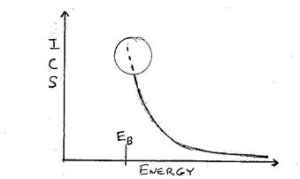
Each element in the sample can only be excited by that part of the source spectrum above the shell binding energy (EB), BUT is most excited by that part of the energy structure near the edge and much less so by that further away.
Therefore “shape” as well as intensity can be of critical importance.
Ideally one should measure the exact x-ray spectrum at the sample position under the same conditions that will be used for sample measurements including
tube voltage, tube current, pre-filters, etc
This however is rarely feasible with most spectrometers due to extremely high incident rates and the lack of opportunity to place a detector in the sample position. Even where this may be possible it requires that the “observed” spectrum be de-convolved back to the “actual” spectrum taking into account such factors as
- the intrinsic detector efficiency
- the energy and spectral dependent line shapes
- the electronic efficiency
For these reasons, FP analytical software usually attempts to define a reasonable approximation of the source spectrum at the sample by means of models of the x-ray tube spectra. There are many such models but two that have been used by analytical software are those by
Pella et. al. (1985) & Ebel et. al. (1992)
However, all models are deficient whenever
- there is incomplete or incorrect knowledge about the exact tube operating parameters [voltage, current, anode material & take off angle, window material and thickness etc]
- there are unknown contaminant characteristic lines in the spectrum
- or simply as the tube ages and changes
This is why the best these models can provide is an approximation of the x-ray spectrum striking the sample which may be quite adequate for some samples and much less so for others.
The FP Physics Database
All of the above calculations depend on the FP physics database which includes a source for such information as:
- x-ray line energies for each Z
- x-ray line relative intensities
- x-ray induced ionization cross-sections
- K, L, M shell and sub-shell fluorescent yields
- Coster-Kronig transition probabilities for the L & M sub-shells
- Cascade probabilities – the probability that a K shell vacancy will result in L & M shell vacancies or an L shell vacancy resulting in an M shell vacancy
- X-ray energy dependent mass attenuation coefficients in every material
- scattering cross-sections
- electron-ionization cross-sections for photoelectric & Auger electrons in the sample or characteristic x-ray production in the tube anode
Equation (1) provides the basis for a standardless FP calculation of elemental concentrations with the accuracy of the conversion to concentration depending on the accuracy of all of the factors discussed previously.
Any deficiency in the spectrometer description, assumed x-ray spectrum striking the sample, or the physics database used to calculate the theoretical yields will translate directly into errors in the calculated C(Z) values.
This is why standards are generally used to validate the assumptions
or calibrate the equipment.
If we analyze one or more standards with known concentrations we can re-arrange Eq (1) to define instrument calibration factors that we will call H(Z)
H(Z) = A(Z,True) / [ C(Z) * Y(Z,M,d,N(E),G) ] (2)
If everything is known perfectly then H(Z) will equal 1 for all Z.
When it is not known perfectly then the departure of H(Z) from 1 represents the instrumental error (or fitting error) at that Z as well as the error that would have arisen in a standardless FP calculation.
Equation (2) is then re-arranged to use the H(Z) values in calculating the sample concentrations via
C(Z) = A(Z,True) / [H(Z) * Y(Z,M,d,N(E),G) ] (3)
Which provides the basis for FP analysis with standards or what we will call
“Hybrid FP”
As the Cambridge Scientific FP EDXRF analysis software (CSXRF) will be used in the Gold Alloy case study to be presented later, a brief description of its handling of the x-ray source spectrum issue and the H(Z) factors is in order.
When no source spectrum is provided the CSXRF program combines a source spectrum model description with the H(Z) determination as follows:
A simple source spectrum model involving 5 parameters is used:
- one for the overall intensity,
- two for the bremsstrahlung spectrum (the end point energy and a shape parameter),
- one for the characteristic line intensity of the anode
- one for the characteristic line intensity of the pre-filter.
Not all parameters need to be varied in the fit each time as often the end point energy is well known, and there may be no characteristic lines from the anode or pre-filter depending on the particular arrangement.
Information is collected from one or more standards and then the source model parameters are fit to the criteria that H(Z) will give the best possible fit to 1.
The main advantage provided by the H(Z) is that it allows for some systematic error in the description of the instrument, as long as the errors are not time, rate or spectral dependent.
In fact, the shape of H(Z) as a function of Z or energy (its systematic departure from 1) is often useful in diagnosing system description errors. One example of this is that of the x-ray absorber whose nominal thickness or density is wrong.
For instance if an absorber’s nominal thickness was wrong we might see the following:
Nominal Thickness Nominal Thickness
Low High
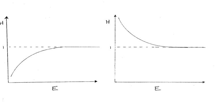
Another example is if the nominal detector crystal thickness is wrong
Low High
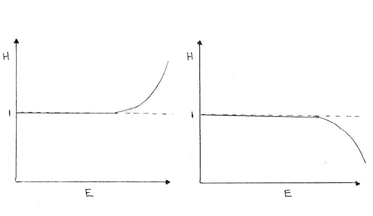
This can make a great deal of difference in the Z and upper energy range where the efficiency is starting to decline exponentially.
In general, small time independent errors can be readily compensated for using Hybrid FP analysis via the H(Z) values.
The more closely the standards match the samples the better the compensation will be.
However, some things are difficult or impossible to compensate for via H(Z).
The obvious condition provides the
1st Necessary Condition for a Robust FP Analysis
You must have a stable instrument
that does not change without your knowledge.
This includes:
- stable geometry
- stable source spectrum
- stable absorber characteristics
- stable detector position and intrinsic efficiency
Another factor that is difficult to compensate for via H(Z) is any time, rate or spectral dependent factors such as the electronic detection efficiency, Delec(Z).
This leads to the
2nd Necessary Condition for Robust FP Analysis
You must have some means of knowing or measuring the electronic efficiency
for each sample spectrum acquired.
This includes:
- the fraction of detected events that represent true x-rays as opposed to noise
- the system dead time
- some means of estimating the number of x-rays lost to discrimination or pile up. This includes partial pile up and pile up with noise.
Most x-ray spectrometers rely on a single measure for the electronic efficiency, namely the
dead time ( or live time) fraction
In many situations this may be sufficient but the ‘robustness’ would be improved by measuring standards similar to the sample with similar live time fractions both before and after each sample checking that the post sample results match the pre sample results.
Although this requires more work and cannot guarantee the sample measurement was done under the same circumstances it is highly suggestive and reassuring.
Even then the robustness could be improved if each measurement, whether standard or sample, gave sufficient information unto itself to make such a determination.
One solution to this problem has been implemented in the Cambridge Scientific CSX line of digital signal processors. It processors all recognized events into one of two spectra:
- the normal processed spectrum of accepted events
- a second spectrum that contains all of the events that were rejected for one reason or another
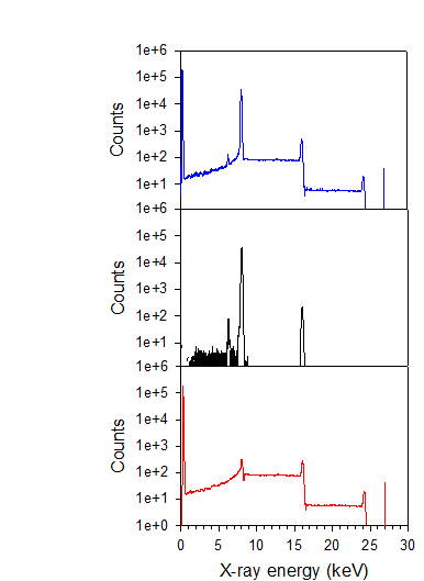
For illustrative purposes we show a simple mono-energetic Cu Ka1 spectrum with the rejected spectrum shown overlapping the accepted event spectrum.
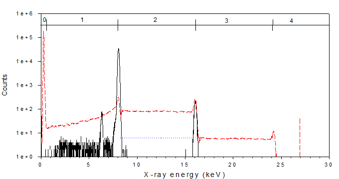 |
The accepted spectrum (solid black line) looks normal with a main peak at about 8 keV, an escape peak, some tailing and a sum peak at 16 keV.
The rejected spectrum (dashed red line) shows many of the same features but also shows features that include
- an additional large noise peak below 1 keV
- a pile up of a single 8keV event with noise in the region below 8 keV
- a pile up plateau between 8 & 16 keV representing the partial pile up of two 8 keV events (a small fraction of these events probably represent the pile up of 3 partial events)
- a pile up region above 16 keV representing the partial pile up of three 8 keV events
The CSXRF program has been designed to take advantage of this extra information provided by the rejected spectrum to determine the true event input rate by subtracting the noise only events and multiplying the pile up events by the appropriate count per event. In this simple spectrum the true input rate can be quite accurately estimated.
Algorithms for estimating the true input rate in more complex spectra have been developed and implemented in the CSXRF program.
The CSX processors also provide a measurement mode for obtaining the interspike time histogram, which can be used to validate assumptions about the Poisson nature of the process. If it is determined that the sample x-rays arrive with a Poisson distribution an analysis of the interval histogram provides another measure of the true input rate.
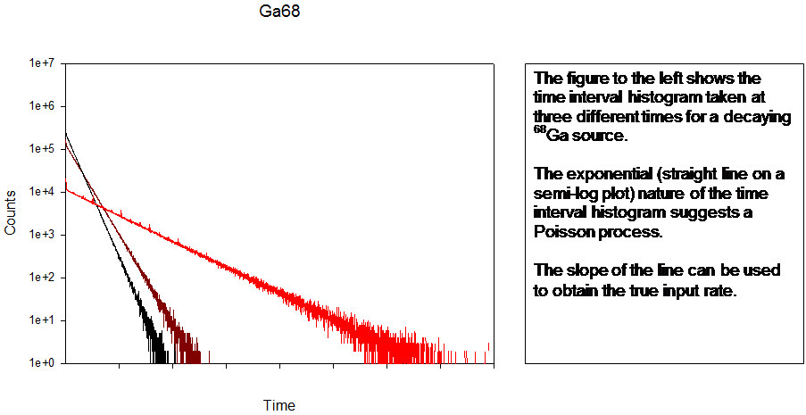
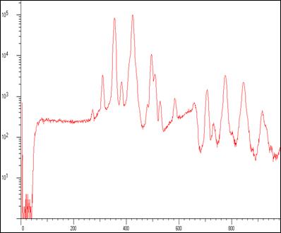
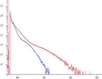
A Pb spectrum (260 kcps input rate) showing Pb L’s and 1st order sum peaks taken on an industrial XRF machine. The interspike time distribution (at two different tube currents) shows non-Poisson behaviour implying that the x-ray tube production fluctuated.
What is the implication?
With most processors the Poisson assumption has to be used to estimate pile up loss and dead time. In this case that would not be possible. However, the CSX rejected event spectrum makes the assumption of Poisson behaviour unnecessary.
So far we have discussed one reason for using standards that are similar in nature to the sample to be measured. That is to provide roughly the same spectral shape and live time in cases where the rejected spectrum is not available for analysis.
Now we present a second reason:
If FP calculated yields depended only on the primary production for each Z then one could measure pure element standards to obtain H(Z) for each element and occasionally measure one or more between samples to make sure conditions are not changing.
However, yields also often depend on secondary processes, the most significant of which is usually secondary fluorescence
- the relative contribution of secondary to primary radiation in Z depends on the distribution of the source x-rays above both the secondary exciter and Z
- this is one reason for using standards that are similar in nature to the samples to be measured
- as the concentration of the secondary fluorescence source atoms changes relative to that of the primary element Z (and change from standard to sample), the spectral shape of the source x-rays becomes more important
This brings us to the:
3rd (Usually) Necessary Condition for Robust FP Analysis
A good representation of the source x-ray spectrum striking the sample.
This includes the overall intensity but is primarily about the spectral shape.
This condition is a little weaker than the first two as there are some sample types where the source x-ray shape is not that important (thin targets, light element sample matrices with no secondary fluorescence, etc)
However in general measurements, where secondary fluorescence contributes to the yield, if the shape is poorly represented then as the sample element concentrations begin to differ from the standard element concentrations the errors will begin to increase and a robust measurement is not possible.
At this point we have specified three necessary conditions for “robust” FP analysis of EDXRF spectra:
1) You must always have a stable instrument
2) You must always have some measure or assurance of the electronic efficiency for each and every measurement
3) You usually have to know the x-ray spectrum striking the sample, particularly the spectral shape
In general we assume that most features of the spectrometer have been reasonably estimated with any small discrepancies taken care of by the instrument calibration factor, H(Z)
Assuming the hybrid approach the "necessary knowledge" conditions vary with the samples to be measured. For example:
- very thin single layers do not require FP for conversion of peak areas to concentration (areal density). The areal densities will scale linearly with the peak area. However, depending on the complexity of the spectrum, they may require FP to accurately determine the element peak areas and well characterized electronics as the true input rate will change as the thickness changes;
- thicker layers require FP corrections since the yield increases asymptotically as the thickness increases and matrix transmission effects as well as possible secondary fluorescence effects come into play in which case the source spectral shape is important;
- measuring sample thickness additionally requires a known source intensity because the counts rely not only on the concentration but also on the areal density and thus rescaling to 100% based on the assumption of a thick target is not an option;
- thick alloys where all elements are visible in the spectrum require FP corrections for thick targets as well as corrections for secondary fluorescence effects and thus require knowledge of the source spectral shape but are independent of the overall intensity as here the results can be scaled to the 100% concentration. If one adds in independent invisible low Z elements then the conditions change again and the intensity once again becomes important;
- RoHS measurements of trace heavy elements (Cd, Pb, Cr, <1ppt) in plastics relies on knowledge of the matrix plastic (type, thickness & density) and the overall intensity of the source spectrum but less so on the shape of the source spectrum as there are no secondary fluorescence effects to be concerned about and transmission effects depend on the high concentration light elements and not the low concentration trace elements;
- layered targets (especially those with unknown thickness) are the toughest test of FP in XRF as they generally require accurate knowledge of all aspects of the measurement system from the source to detector and are often difficult to provide a good standard for corrections of improper assumptions.
-
FP Software
The final component in FP analysis is the software used to obtain the element peak areas from the spectrum and convert those to concentrations.
With the caveat that the complexity and necessary features of the software may depend on the types of analysis to be done; in general the necessary conditions for the analysis software will include:
- a means of identifying and accurately determining the spectral peak areas of the principal lines associated with each element;
- an accurate or at least self-consistent data base used to determine theoretical yields and x-ray attenuation;
- an adequate algorithm for doing the calculations that are important to the types of samples you are measuring;
- if you have no certain knowledge of the source excitation spectrum striking the sample then the software has to be provided with or be able to calculate an adequate approximation of the excitation spectrum;
- a means of determining the ``adjusted peak areas``, that is the spectral peak areas adjusted for such things as x-ray filters, the intrinsic detection efficiency including solid angle and line shape as well as the electronic efficiency which has to account for all events lost from the spectrum due to dead times, pileup & processor discrimination;
- in hybrid analysis, where standards are measured, the correction factors to be applied to each element of the sample analysis have to be calculated, stored and then used to convert the adjusted peak areas of the sample spectra to concentration values via the FP theoretical yield calculation.
This suggests a
4th Necessary Condition for Robust FP Analysis
A software package adequate to the needs
of the measurement being done.
Several packages are in use but the one we use here is the Cambridge Scientific FP EDXRF analysis program – CSXRF.
A brief description of this software is given below.
The CSXRF Software Package
The CSXRF software package is a fundamental parameter (FP) based XRF spectrum analysis program that can be used to analyze x-ray spectra from:
- thin samples to obtain areal densities in mg/cm2
- thick or bulk samples to obtain element concentrations in ppm
- intermediate targets to determine thickness and element concentrations in ppm
- layered targets for layer thickness and element concentrations in ppm
It uses a non-linear least squares (NLLS) procedure to fit a digitally filtered model spectrum to the digitally filtered acquired spectrum in order to:
- find the peak areas of the principal lines of each element visible in the spectrum
- determine the adjusted peak areas based on the equipment description
- convert the adjusted peak areas to element concentrations via a FP based theoretical yield calculation
Spectrum fitting is accomplished in the following manner:
- a library of x-ray line energies and a two-parameter energy calibration is used to locate each peak in the spectrum
- two additional parameters are used to model the energy dependent peak widths
- each peak is modeled as a Gaussian at low intensities or a Voigtian at higher intensities with the Lorentzian widths obtained from the FP database
- each peak also has an associated escape peak and can also be provided with a fixed parameterized tailing structure if so desired
- each element line series (K, L, M) is represented by the intensity of the principal line of that series with all other lines tied to that principal line via a library of relative line intensities adjusted for differential absorption, detection efficiency and thick target effects. If so desired the line series for the K lines can be further divided into Ka & Kb and the L lines can be divided into their sub-shell components L1, L2 & L3.
- the slowly varying background component is not modeled but is instead effectively handled by means of a digital filter
- a non linear least squares procedure (NLLS) is used to fit the digitally filtered model spectrum to the digitally filtered data spectrum
The CSXRF program operates in various modes including:
- fixed matrix (FM) calculation mode, where the element peak areas are calculated and converted to concentrations using a known matrix
- iterated matrix (IM) mode where the element peak areas are calculated and an iterative procedure is used to determine the matrix element concentrations. In this mode invisible elements are handled on the basis that they are dependent or chemically tied to the visible elements (eg. a metallic oxide) or they are independent (eg. water in a hydrated material). If independent then its concentration is considered to be the leftover amount after each iteration of the visible matrix elements
- standard acquisition mode where information on the adjusted peak areas from a sample being used as a standard is calculated and stored along with a vector of theoretical yields versus excitation energy
- instrument calibration mode where the stored standard information is used to calculate the instrument calibration values H(Z) and if necessary estimate the shape and intensity of the x-ray source spectrum at the sample
Case Study: Gold Alloys
In this case an OEM was using the CSXRF software for the purpose of obtaining the concentration of elements in gold alloys using their own spectrometer system. Here we are looking at alloys consisting of up to four elements, Au, Ag, Cu, Zn, all of which provide visible x-ray peaks in the spectrum and whose concentrations must sum to 1.
This fits the general case of having to know the spectral shape of the source x-rays striking the sample but not the actual intensity. Variation of the tube current does not matter as long as it DOES NOT alter the spectral shape. It is up to the manufacturer or analyst to confirm that for their equipment.
As the OEM does not provide an x-ray tube excitation spectrum for their various configurations of different tubes, anodes and primary filters it was necessary for the FP program to estimate the spectral shape based on the minimal information provided by the equipment manufacturer including anode Z, window material and thickness and primary filter Z and thickness.
The table to follow shows the results of their analysis of 60-second measurements of 20 gold alloy standards. The spectra were generated using an W anode x-ray tube and 50 mm Ta primary filter and collected using a 13 mm2 400 mm thick Moxtek SiPin using the OEM’s signal processor. Although no counts or errors are listed the FP analysis provides good agreement.
Of particular note is that low concentration Zn is difficult to measure in a high concentration Au/Cu sample because the Zn Ka overlaps with the Au Ll line as well as the Cu Kb lines and the scattered x-ray tube W anode characteristic radiation and the Zn Kb lies on the leading edge of the Au La peak.
Also the Ta primary filter, with L3 edge at about 9.9 keV although good for suppressing the bremsstrahlung radiation from the tube in the Au Lb & Au Lg region is not as effective in the energy range below 9.9 where the Cu, Zn & Au La peaks reside. Longer measurements (or higher count rates) in order to provide greater statistical accuracy may be required in order to obtain better Zn values in these cases.
Measured values Certified Values
FP Analysis of 20 Gold Alloy Standards
Au
Ag Cu
Zn
Au Ag
Cu Zn Total
1 99.754 0.161 0.049 0.036 99.71 0.14 0.15 0.00 100.00
2 99.611 0.334 0.052 0.0 99.58 0.30 0.12 0.00 100.00
3 99.438 0.540 0.071 0.0 99.32 0.52 0.16 0.00 100.00
4 98.940 1.060 0.0 0.0 98.87 1.02 0.11 0.00 100.00
5 91.688 8.312 0.0 0.0 91.57 8.25 0.16 0.02 100.00
6 85.119 13.748 1.133 0.0 85.19 13.76 1.03 0.02 100.00
7 80.168 17.807 2.024 0.0 80.18 17.82 2.00 0.00 100.00
8 74.606 12.147 11.588 1.659 75.10 12.34 11.57 0.99 100.00
9 69.439 8.928 20.281 1.348 70.21 9.21 19.60 0.98 100.00
10 64.396 10.442 23.362 1.793 64.95 10.75 22.88 1.42 100.00
11 58.492 20.510 20.999 0.0 58.42 21.18 20.31 0.09 100.00
12 58.513 26.745 14.745 0.0 58.45 27.15 14.40 0.00 100.00
13 58.679 24.660 15.025 1.634 58.64 24.59 15.18 1.59 100.00
14 58.335 36.949 28.515 9.455 59.48 4.20 27.33 8.99 100.00
15 55.035 12.820 29.431 2.713 55.17 13.65 29.15 2.03 100.00
16 50.539 14.628 33.319 1.512 50.45 15.38 33.02 1.15 100.00
17 45.518 16.380 36.161 1.941 45.70 16.41 36.30 1.59 100.00
18 41.021 17.057 39.340 2.582 41.70 17.89 38.39 2.02 100.00
19 34.989 18.483 43.705 2.822 35.32 19.95 42.80 1.93 100.00
20 33.403 18.574 46.585 1.437 33.53 19.75 45.74 0.98 100.00
For the table above the procedure would have been as follows:
- one alloy was chosen as a standard (#13) and the other 19 were run as samples producing a total of 20 spectra all at the same tube voltage
- the standard spectrum was analyzed in FM (fixed matrix) mode for the peak areas of the element lines and this information was used by the program along with theoretical yield calculations to estimate the shape and intensity of the x-ray spectrum striking the sample as well as to produce a table of H(Z) values for the certified elements with the results stored in files
- this generated excitation file along with the H(Z) value files were then used to analyze the sample spectra in IM (iterative matrix) mode to produce a table of concentration values that we see in the above table. In iterative matrix mode the sample matrix composition is iterated (and in this case scaled such that the concentrations summed to 1) until the results converge.
Although we were not provided with the spectral data files that resulted in the table we were provided with a few spectrum of these gold alloy materials collected at a prior time using this system and reported these analyses back to the OEM for their action. Spectra for 1, 13 & 14 were obtained and analyzed with some of the results and comments reported below. We analyzed #13 and used that spectrum as the standard for analyzing #1 & #14 as well as reanalyzing #13 to ensure self-consistency in the calculation.
One of the numbers reported by the CSXRF code in IM mode, in the case where all of the elements produce peaks in the spectra, is the H correction factor.
This factor is the scale factor that is required to multiply all H values in order for the concentrations to sum to 1.
Since #13 was used as the standard to produce the excitation spectrum and the H(Z) values its H correction factor is 1. This is a useful cross check.
However, the H correction factors for the #1 and #14 samples were 1.32 and 1.42 respectively.
Case Conclusion:
The constraint of the concentrations summing to 1 allowed useful analyses for gold alloys (and by extension to similar types of systems where the sum of the visible elements and any associated invisible elements must sum to 1).
In this case the widely varying H correction factor indicates that the equipment has one or more problems that need to be addressed before proceeding to more complicated analyses. This is what we reported back to the OEM for their action.
Last, but certainly not least,
The Final Necessary Condition for Robust FP Analysis
An analyst who is willing to do more
than simply push a button and record a result.
General Good Practices
A list of good practices (certainly not complete) for the analyst to keep in mind include such things as:
- standards should be run to higher than normal statistics in order to reduce the statistical error in the standard element fits that translates directly into errors in the associated H(Z) values. Remember most software packages will report errors in the fitted peak but have no idea about systematic errors or errors in the calibration constants.
- reanalyze the standard spectrum as a fixed matrix sample to ensure that you are using the right excitation and H(Z) files.
- if reported by the software, observe the contents of the H(Z) , detection efficiency and absorber transmission values for each element in order to determine how sensitive the results may be to systematic errors in the description of the equipment or the generated excitation file
- analyze standards frequently and compare results to previous analyses to make sure the spectrometer or analysis is not changing with time
- for any given set of standard and sample measurements the x-ray tube voltage should remain constant as changing the tube voltage would change the x-ray spectrum shape. Even changing the tube current in order to change the source intensity should be approached with caution and its effects investigated on your spectrometer.
Analysts should know their instrument and software
and have a basic understanding of the technique
so that they can recognize problems
and deal with them appropriately.
Summary & Discussion
In pure standardless FP analysis every aspect of the spectrometer system must be well known. In Hybrid FP analysis the use of standards to characterize the instrument compensates for some inaccuracies in the system description.
However, even in the case of Hybrid FP, there are certain irreducible necessary conditions for repeatable and accurate (robust) FP analyses of EDXRF spectra. These include:
- Stable equipment that can provide repeatable measurements
- Some means of determining the true x-ray input rate
- Knowledge of the shape and/or intensity of the spectrum of x-rays striking the sample
- Some knowledge of the sample and any necessary sample preparation
- A software package adequate to the needs of the given analysis
- A “good” analyst, who practices good techniques and knows his instrument
Additional knowledge may be required depending on the type of sample being analyzed.
Ideally every aspect of the measurement system is well characterized, a suitable standard is available for system checks and an adequate software package is available for the analyses. However this is generally not the case and this is why we have to evaluate the robustness of a particular FP analysis system from the measurement apparatus to the FP analysis code for each type of measurement to be done.